Encountering Massive Activations in Gemma 3

Dimensions 1038, 443 and 2339 in Gemma 3 1B, 4B and 12B models.

TL;DR: While working with Gemma 3 models , I encountered “massive activation” dimensions whose magnitudes are about 2,000$\times$ the median value. At the layer I analyzed, I found exactly one such dimension per model in Gemma 3 1B, 4B, and 12B, but none in Qwen or Llama . These massive activations don’t seem to have any causal importance, but their values distort representational analysis by inflating cosine similarity, making every vector appear to point in the same direction.

Preliminaries

Transformers. LLMs are typically decoder-only transformers , with many layers of transformer blocks stacked one after another. These models take in a sequence of text, tokenize it, and convert each token into a high-dimensional embedding vector in $\mathbb{R}^{d_{model}}$. For a sequence of $n$ tokens, this gives $X \in \mathbb{R}^{n \times d_{model}}$.

The residual stream. Conceptually, an LLM can be thought of as a multi-layer model that reads representations, computes and applies updates to them, and then reads the final representations to produce the output. In particular, a transformer block, which itself contains an attention layer and a feed-forward layer, reads from these embeddings, performs some black-box computation, then applies the change to the input embeddings via a residual connection. We call the output of a transformer block an activation vector $h_l \in \mathbb{R}^{d_{model}}$. The outputs of all layers are also called the “residual stream” , because information gets read from and written to this stream (Figure 1). Note that $X$ is also $h_0$, i.e., the token embedding is the first step in the residual stream.

Interpretability. It turns out that activation vectors are not mere numbers; they contain information about what the LLM has learned, i.e., how models “represent” the input data. That is to say, if we read the activation vectors, we can identify geometric structures that correspond to human concepts. So, we also sometimes refer to activation vectors as “model representations”, especially if we can find specific vectors that seem to represent actual concepts.

Representation and Steering

Linear representations. The most popular realization of this idea is the linear representation hypothesis , which says that LLMs represent concepts as linear directions, i.e., a single vector. The implication of this is that we can use simple vector arithmetic to manipulate and control LLM behavior.

Linear activation steering. Let’s say the model is processing some negative input $X^{neg}$, has some negative representation $h^{neg}$, and outputs some negative token $Y^{neg}$, but we want a positive output instead. We can directly intervene on $h$ by adding a steering vector $v^{neg \rightarrow pos}$ which points from negative to positive, so that $h^{neg} + v \rightarrow h^{pos}$. The later layers will then read from this representation and produce the positive output $Y^{pos}$ (Figure 2). In practice, this typically works well for concepts that have clear opposites, such as harmful → harmless, or hate → love, but less well for concepts with no clear polarity, such as numbers.

This activation steering technique is what I’m working with. To sum up, we can manipulate a model’s behavior by directly changing its activation vector, and we can do this by adding a steering vector. How the steering vector is computed is another topic, but typically it’s a difference-in-means over some dataset, as in Contrastive Activation Addition (CAA) .

Representation analysis. Another thing we can do is measure how similarly an LLM represents two concepts. We would reasonably expect model representations to reflect the real world. For example, if we take the representations for coffee and tea, we would expect their similarity to be higher than, say, between coffee and bread, but lower than between coffee and cà phê (the Vietnamese word for coffee). We typically measure similarity using cosine similarity, which ranges from −1 to 1. The closer cosine is to 1, the more similar the representations; 0 means unrelated (orthogonal), and −1 means they point in opposite directions.

Massive Activations

A recent project of mine involved comparing steering vectors extracted from different languages. My first thought was to compute their cosine similarity. I was expecting to find that LLMs use roughly the same direction to represent a concept across languages, which is a known finding . That is to say, the cosine similarity between $h^{\text{coffee}}$, $h^{\text{cà phê}}$, and $h^{\text{café}}$ would be close to 1.

When I did this on Gemma 3 4B and 12B, I got exactly this: cosine ≈ 0.96. It seemed like the models represented my studied concept in the same direction across languages after all.

Except that was not what was happening.

Why wasn’t that the case?

At first, the results looked suspicious because the cosine for Gemma 3 4B and 12B specifically was very high, while Gemma 3 1B, Qwen, and Llama were in the 0.5–0.7 range.

And then, an LLM I used to proofread a paper draft suggested that the high cosine could have been inflated by extremely large activation values in some of the dimensions, which, unbeknownst to me at the time, was a known phenomenon in the literature . These massive activations are simply values that are several thousand times larger than the typical activation value, and they carry most of the magnitude of the activation vector (i.e., $|h|$). Similar “outlier” or “rogue” dimensions were also reported in earlier models such as BERT and GPT-2 .

Below, I’ll outline how they affected my experiments. For context, in the paper’s setup I was only working with one layer per model. So, these massive activations could pop up in other layers too—I haven’t checked because it’s irrelevant to my paper.

Finding massive activation dimensions

I ranked dimensions by their mean absolute value across languages, and compared the top-ranked dimension with the median dimension. I found exactly one such dimension per model in the Gemma family, but none in the other models (Table 1).

Model	Dimension	Ratio to median	Share of squared length
Gemma 3 1B	1038	525×	0.2–52.7%
Gemma 3 4B	443	2,093×	85.5–92.6%
Gemma 3 12B	2339	2,198×	83.9–93.2%
Qwen3 4B	0	54×	0.1–3.8%
Qwen3.5 9B	3994	166×	0.0–1.3%
Llama 3.1 8B	4055	38×	0.1–1.9%

Table 1. The top-ranked dimension of the steering vectors in each model. “Ratio to median” compares its mean absolute value to the median dimension. “Share of squared length” is the fraction of the vector’s squared norm that this one dimension carries, across the four languages.

In Gemma 3 4B and 12B, this one dimension carries around 90% of the steering vector’s squared length. In Gemma 3 1B, it is large in some languages but small in others. In Qwen and Llama, the top dimension carries at most a few percent.

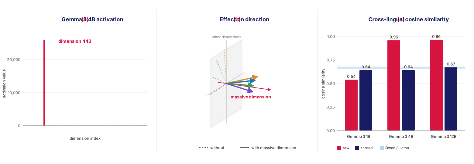
The massive dimension is not only in the steering vectors; it is already in the model’s activations. For example, dimension 443 in Gemma 3 4B’s layer 13 has an activation value of about 26,000, roughly 2,600$\times$ the median absolute value (Figure 3). This is so large that if we plot it on a linear scale, it dwarfs every other dimension. Only after setting it to 0 and zooming in can we see the rest of the vector.

Why massive activations inflate cosine similarity

Cosine similarity only looks at the direction of two vectors, not their length:

\[\cos(a, b) = \frac{a \cdot b}{\|a\| \, \|b\|}\]

If two vectors share one huge dimension, that dimension dominates both the numerator and the denominator. Both vectors then point almost entirely along that one axis, and the cosine ends up close to 1, no matter what the other dimensions say.

As a toy example, take $a = [1000, 1, 2]$ and $b = [1000, -2, 1]$. If we ignore the first dimension, $[1, 2]$ and $[-2, 1]$ are orthogonal, i.e., cosine = 0. But with the first dimension included, cosine = $10^6 / (10^6 + 5) \approx 0.99999$. Figure 4a shows this in 3D: the larger the massive dimension, the more both vectors lean toward its axis, and the smaller the angle between them.

The massive dimension can also do the opposite. If it is large in one vector but small in the other, the two vectors point in different directions and the cosine is pulled down. This is what happens in Gemma 3 1B.

Dealing with massive activations

One way to examine the role of these massive activations is to set their values to 0. That is, we create a new vector $v^{\perp}$ by zeroing out the massive dimension $i$ of $v$, so that $v^{\perp}$ is orthogonal to the basis vector $e_i$ of that dimension.

First, I tested whether zeroing out these dimensions had any effect on my steering experiments. Here, I also rescaled $v^{\perp}$ to the norm of the original $v$, so that the steering strength would remain the same. Overall, the steering results were roughly the same before and after zeroing: the flip rate (how often steering flips the model’s output) changed by less than 1 percentage point on average, and by at most 4 percentage points (Table 2).

Model	Mean change in flip rate	Max change in flip rate
Gemma 3 1B	0.7 pp	3 pp
Gemma 3 4B	0.4 pp	2 pp
Gemma 3 12B	0.5 pp	4 pp

Table 2. Change in steering results after zeroing the massive dimension, across all within-language and cross-language settings.

Second, I recomputed cosine similarity. This time, the cross-language cosine similarity of Gemma models was much more in line with Qwen and Llama (Figure 4b). Perhaps surprisingly, they all landed in the 0.64–0.68 range. Note that for Gemma 3 1B, the cosine actually went up (0.540 → 0.642), because its massive dimension was large in some languages but small in others.

Conclusion

Massive activations are a bizarre phenomenon for two reasons. First, they are very specific: they only surface in one dimension per model, and only in Gemma models but not in the others I tested. Second, they have virtually no causal effect on steering (the models work fine, and steering interventions succeed with or without them), and they only surface as an issue when comparing representations. I leave the origin and the broader effects of these dimensions to future work. In my case, I simply zero them out to isolate their impact on the similarity analysis.